Applications in Engineering & Control Systems

Why transforms matter in engineering

Transforms are operational levers: they replace differentiation and convolution with algebraic multiplication and division, making linear time-invariant (LTI) models tractable. Transfer functions are rational functions in the complex variable s; poles determine natural response and stability, and zeros influence transient shape and steady-state gains. Convolution of an input with an impulse response becomes multiplication of the input transform by the transfer function—this simplifies system-level interconnections and control-loop analysis.

Common engineering workflows that use Laplace

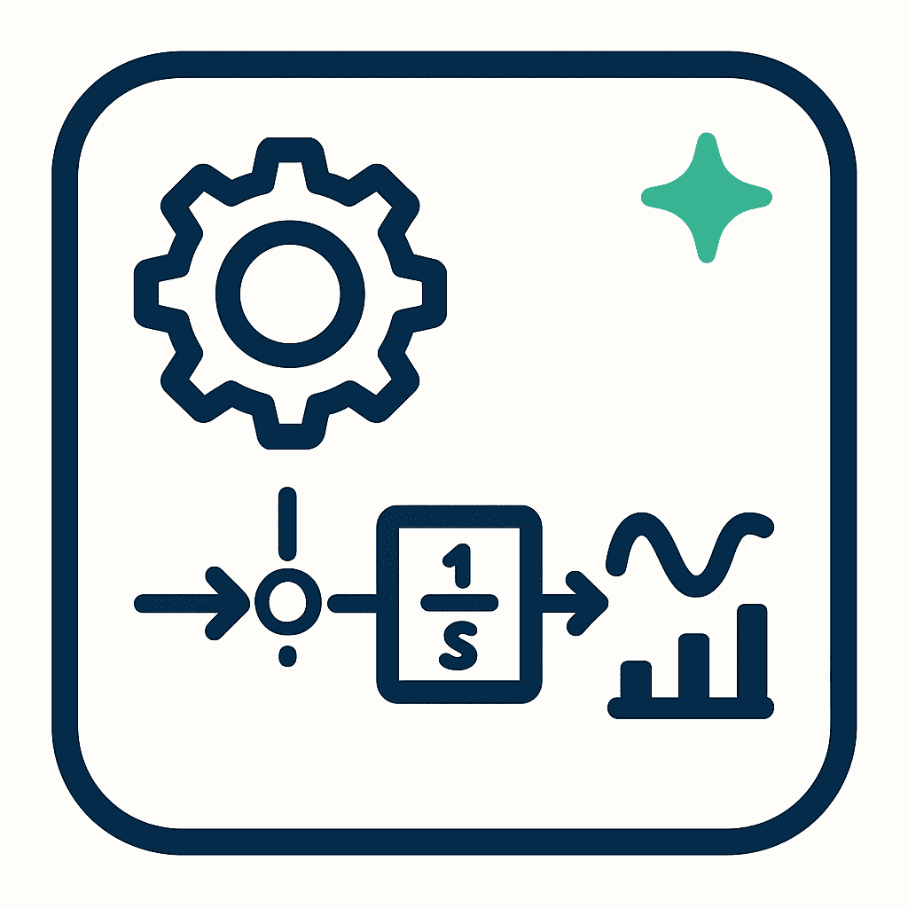
• System identification and linear modelling. Empirical or first-principles ODEs are converted to transfer functions using the Laplace transform for subsequent design. Use a laplace transform for differential equations pattern (replace derivatives with s-multipliers and include initial conditions) to build the s-domain model.
• Controller design (PID, lead/lag, root locus). The s-domain representation is primary: Bode and Nyquist plots are created from transfer functions to assess gain and phase margins. A laplace s-domain calculator embedded in control toolboxes automates the conversion between time-domain ODEs and transfer functions.
• Transient and stability analysis. Compute impulse and step responses using analytic inversion or a laplace transform table lookup for canonical terms. For switched or delayed signals, the laplace of unit step function and shifting properties form causal expressions.
• Block diagram algebra and model reduction. Series, parallel and feedback interconnections are reduced algebraically in the s-domain; model-order reduction techniques simplify high-order models while preserving dominant poles.
• Signal conditioning and filtering. Laplace-based transfer functions provide controller-compatible filter designs; simulation environments offer a signal processing laplace tool to link continuous-time filters to discrete implementations.

Representative worked patterns

• From ODE to transfer function. Given a linear ODE with zero initial conditions, apply the Laplace transform, factor polynomials, and express output/input as Y(s)/U(s). This ratio is the plant transfer function used in controller design.
• Step-response specification. Designers select controller gains so closed-loop poles place natural frequency and damping ratio at target values; invert using a symbolic inverse laplace transform solver or a table lookup when expressions are complex.
• Handling nonzero initial conditions. Use the full transform rules (terms like sF(s) − f(0⁺)) to include initial transients in simulation and test validation.

Tools and verification: practice and automation

Engineers should use a combination of symbolic, numeric and measurement tools:

• Symbolic verification and teaching. A laplace transform step-by-step engine or CAS (SymPy, Mathematica) helps verify algebraic manipulations and partial-fraction inversions; a laplace transform practice solver supports classroom and self-study validation. See SymPy: https://www.sympy.org/.
• Rapid prototyping. A laplace transform calculator online and a laplace s-domain calculator embedded in MATLAB/Octave or Python’s control and scipy.signal packages provide quick conversions from ODEs to transfer functions and compute responses numerically. See SciPy signal docs: https://docs.scipy.org/doc/scipy/reference/signal.html.
• Numeric inversion and edge cases. For complex rational expressions with high-order poles, an inverse laplace transform solver (symbolic or numeric) provides a robust inversion path; numerical Bromwich or Talbot implementations are employed where closed-form inversion is impractical.
• Measurement cross-checks. Validate analytic predictions with measured step/impulse responses and frequency sweeps. Compare measured FRFs to transfer functions obtained via Laplace methods and update models to account for unmodelled dynamics.

Examples drawn from domains

• Power systems. Small-signal stability analysis linearises generator and converter models; Laplace-domain transfer functions are used for eigenvalue (pole) placement and controller tuning.
• Aerospace. Guidance and autopilot loops use s-domain models for phase-margin-based robustness and for deriving lead–lag compensators.
• Process control. Chemical plants use PID controllers derived from first-order-plus-dead-time approximations; the laplace of unit step function is used to compute setpoint responses and tuning rules.

Numerical and practical cautions

• Numerical inversion sensitivity. When using an inverse laplace transform solver numerically, ensure algorithms and precision settings are adequate; validate results by forward-transforming the time response back to the s-domain at selected complex frequencies.
• Causality and model validity. Laplace methods assume linearity and time invariance. For nonlinear or time-varying systems, linearise around operating points and treat Laplace-domain models as local approximations.
• Discretisation. When controllers are implemented digitally, convert continuous s-domain designs to z-domain equivalents using bilinear transform or matched-pole techniques and verify frequency-domain behaviour with FFT-based tests.

Useful references and teaching materials

• MIT OpenCourseWare lecture notes and exercises summarise the algebraic advantage of Laplace transforms for ODEs and control-model generation: https://ocw.mit.edu/courses/.
• Standard control texts provide design methods, pole-placement theory and practical tuning recipes; use those texts alongside symbolic tools for reproducible designs.

How to incorporate transform tools into a workflow

1. Model derivation (ODE).
2. Laplace apply and algebra (use a laplace transform table lookup or laplace transform step-by-step if uncertain).
3. Transfer function formation via a laplace s-domain calculator.
4. Controller design (root-locus/Bode).
5. Inverse transform via symbolic solver or inverse laplace transform solver to produce time-domain predictions.
6. Measurement validation and iterative model refinement (instrumented step tests, FFT analysis).

Final Considerations

Engineering practice treats Laplace transforms as a bridge between differential models and algebraic methods for analysis, design and verification. The s-domain representation is the lingua franca of classical control: it supports transfer-function algebra, stability margins, and transient-specification mapping. Practitioners should pair concise analytic techniques (use a laplace transform table lookup to recognise canonical inverses and compute laplace of sin t or the laplace of unit step function when modelling inputs) with robust tooling (a laplace transform calculator online, laplace transform practice solver, and an inverse laplace transform solver). Verification—both symbolic and measured—completes the loop: forward-transform time responses, compare with measured FRFs, and adjust models to reflect real-world dynamics. This disciplined stack reduces design risk, clarifies the trade-offs between robustness and performance, and supports reproducible controller deployments across mechanical, electrical and process-engineering domains.